Mountain flying: unconsidered factors

by Thomas P. Turner

Even on the flattest continent in the world, mountains exert an influence that pilots must understand.

I’ve been fortunate to fly as a guest of Australian friends in light aeroplanes up and down Australia’s east coast from Maroochydore and Archerfield as far south as Port Macquarie, southwest to Canberra, Melbourne and Moorabbin, up to Cowra and Armidale, and out-and-back to Uluru via Longreach, Birdsville, Oodnadatta and White Cliffs. Except for the wide stretches over the desert Outback, one thing that strikes me about flying in Australia is that you are never far from the aerial influence of mountains. There are several factors to take into account when engaged in mountain and near-mountain flying. Let’s look at some of the performance effects you must consider.

Density altitude

Barring precise pilot’s operating handbook performance data for your aeroplane at various altitudes, you may approximate the impact of density altitude on aeroplane performance by using the Koch Chart (figure 1). Substitute 1013.2 hectoPascals for the 29.92 inches of mercury altimeter setting to find the pressure altitude. Draw a line from the ambient temperature at the left to the pressure altitude at the right. This line passes through factors to multiply with sea level performance to derive aeroplane performance under the higher density altitude condition. In the illustrated example, for instance, on a 38 degrees Celsius day at an airport 6000 feet above sea level, the take-off distance will be roughly 3.3 times greater than at sea level an 15 degrees Celsius, while climb rate will be only 25 per cent of the maximum climb rate available at sea level on a standard day.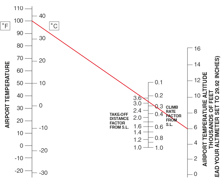

Unlike the United States, where this chart was published, Australia does not have 6000-foot MSL airports. You can see, however, that even at the elevations you can encounter in Australia, when the temperature is high, the aeroplane performance impact is striking.

We usually only think about density altitude in the context of taking off from a hot and/or high-elevation aerodrome. Consider the pilot, however, flying fairly low when encountering the need to climb to avoid terrain. The take-off distance impact of the Koch chart has no relevance in this case. But the rate-of-climb information may be vital to clearing the height of a ridge. Any time you’re flying near rising terrain, consider the density altitude impact on climb performance. Begin your climb early to avoid a condition when the hills have a steeper climb gradient than your aircraft.

True airspeed

The higher the density altitude, the less dense the atmosphere. This means that for a given rate of passage through space—your true airspeed—the fewer molecules of air will enter the aeroplane’s pitot tube per unit of time. Another way of thinking about this is to say on a normal day at sea level you may have to move forward 300 metres to hit enough air molecules to create enough pressure in the pitot system to register as 60 knots on the airspeed indicator, but that on a hot day you might have to travel 400 metres to hit enough air molecules to give you that 60 knot indication. What this means is that the higher the density altitude, the greater the true airspeed must be in order to create a given indicated airspeed.

Because you need a certain amount of air over the wings to attain desired aircraft performance, such as take-off or landing, you must fly the same indicated airspeeds regardless of altitude or temperature. At higher density altitudes, however, this means you will be at a higher true airspeed when you do so. On take-off, it will take longer to accelerate to the higher true airspeed in order to see the required indicated airspeed—you’ll use more runway to take off, and require more horizontal distance to climb. When landing, your higher true airspeed at the proper indicated final approach speed means you’ll touch down with more inertia than you have at lower density altitudes; even if you fly the correct indicated airspeed and do not float excessively during your landing flare, you’ll still use more runway in order to come to a stop.

Where this can really get a pilot into trouble is if you don’t trust the indicated airspeed, and try to fly your circuit and landing entirely by the appearance of the ground as it rushes past, and the runway as it appears to move toward you on your final approach. With a faster-than-normal true airspeed your ground references will tempt you to slow the aeroplane excessively. Because of the higher true airspeed your turns from downwind to base leg, and from base to final, will generate a wider turning radius; if you subconsciously tighten the turn to make the ground references look ‘normal’ you will add load up the wing with G-load and risk an accelerated stall.

So, fly the proper indicated airspeeds in the circuit in the mountains, but expect wider turning radiuses and the need for longer take-off and landing rolls.

Mechanical turbulence

Imagine wading along a shallow but fast-moving stream. Looking into the clear, rushing water, you can see how it forms eddies and turbulent flows as the water passes rocks on the stream bed. Leaves and bubbles in the stream speed up and slow down, bounce, and rapidly change direction and height as they encounter the burbles of water.

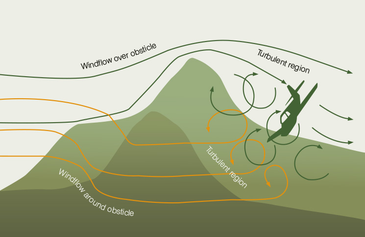
Air around rising terrain behaves just like water in a swift-flowing stream. The phenomenon is called mechanical turbulence (figure 2). Swift airflow around hills can accelerate in venturi-like canyons and valleys. It will change direction rapidly, both vertically and laterally, and may create eddies and even reverse flow patterns. Visualise the air flowing around mountains as if it was visible water flowing over rocks in a riverbed, and you’ll see how potentially hazardous flying near mountains can be when swift winds are blowing.

Mountain wave

An ATSB accident report from the helicopter crash that killed entertainer Graeme ‘Shirley’ Strachan in August 2001 includes this warning:

‘In Australia mountain waves are experienced over and on the lee side of mountain ranges in the south-east of the continent and in westerly wind flows over the east coast in late winter and early spring. It is absolutely essential that aviators are aware of the wind and its potential effects on aircraft. We hope that out of this tragedy, a greater pilot awareness of mountain waves will save lives in the future.’

Mountain waves are a unique phenomenon, different from ‘simple’ mountain-related mechanical turbulence. Mountain waves can be benign, or they may be extremely hazardous—and it may not always be possible to tell which before entering a hazardous zone.

For a mountain wave to form all three of these factors must be present:

• The air mass over the mountains is very stable
• The wind at the height of the ridge or mountain tops must be blowing more than about 25 knots
• The flow of wind at the ridge or mountaintop height must be roughly perpendicular to the ridge.

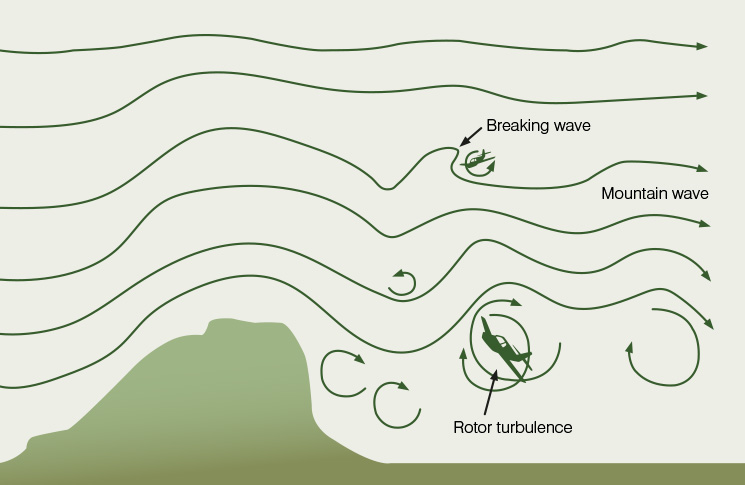
When a mountain wave forms, wind hitting the ridge is deflected upward (figure 3). As it climbs the air cools, becoming denser; the heavier weight of cool air forces it downward toward the surface. The accelerating airflow warms and rebounds off the surface, rising again and repeating the cycle. Seen from the side, this looks like waves hitting a beach. Depending on the initial speed of the wind, the level of atmospheric stability, and the quality of terrain on the leeward side of the mountains, the mountain wave may extend as much as hundreds of kilometres.

The ATSB tells us: ‘If the wave amplitude is large enough, then the waves become unstable and break, similar to the breaking waves seen in the surf. Within these “breaking waves”, the atmospheric flow becomes turbulent.’ In the parts of the wave where the wind separates from the ridge, and above where it rebounds off the surface, intense vortices or ‘rotors’ can form. ‘Breaking waves and rotors associated with mountain waves are among the most hazardous phenomenon [sic] that pilots can experience,’ reports the ATSB. Upward and downward rates of airflow can exceed 8000 feet per minute, more than any light aeroplane can outclimb if caught in the downwind.

Glider pilots love mountain waves; they can ride the rising waves to remain aloft for long periods, often soaring perpendicular to mountain ridges on the leeward side to remain in the upward flow for long times, or over long distances. Pilots of powered aeroplanes can do the same thing. But powered aeroplane pilots generally do not want to go where the wind flow permits, they want to go to where the pilot wants to be. Consequently powered aeroplane pilots are not usually content to remain in the upward part of a mountain wave, and eventually find themselves in the strong downward flow or possibly a breaking wave or rotor. Generally, mountain wave conditions are to be avoided in powered aeroplanes because of the extreme hazards you are likely to encounter.

Mountain wave conditions may sometimes be identified by lens-shaped or lenticular clouds that form at the crests of the wavelike flow. Because lenticular clouds do not move over the terrain, they are sometimes called standing lenticulars. Lenticular clouds form when there is sufficient moisture in the air to reach the point of condensation when the air cools at the top of the waves. From there descending air warms until the air is no longer saturated. It’s not that the moist air is trapped in a fixed spot over the grounds; it’s that the air over that point is at the temperature of condensation, and the air is warmer at other parts of the wave. Consider a single parcel of moist air. It is vapour as it rises off the ridge, becomes visible condensation at the top of the wave, and returns to vapour as it descends. The lenticular cloud is constantly fed new, moist air that exists as visible cloud only for a short time.

Unconsidered factors

Australian pilots may not log a lot of take-offs and landings from mountain airports, but they very frequently fly over or near mountains, and in areas affected by the influence of mountains on the surrounding air. Some of the phenomena that may seem to be merely the realm of theory—density altitude, the difference between indicated and true airspeed, mechanical turbulence and mountain waves—may have very practical, real-world application to Australian flying. Consider the impact of heat and altitude on aeroplane performance, and visualise the flow of air around and above terrain, especially when the winds are strong and when the air is stable.